bilíngue · en / pt
um pytorch onde erro de shape não compila
On September 29, Taelin, the creator of Bend, published a long info dump about the language's future. His company was raising a funding round, was going to set up two new teams, and in the middle of the text there was a wishlist for the ecosystem. One item on the list read: "AI framework / PyTorch / llama.bend / etc.".
Someone asked, in the replies, what a person should do to join one of those teams. The answer was short: build something in Bend, something that shows investors traction and impresses the team.
I had already written about the language's idea and built the editor extensions. What was missing was using it for real, on something big. So I took that wishlist item and spent October 3 and 4 on it. The result is called bend-ml: a machine learning library in Bend, five published packages, a handwritten-digit classifier and GPT-2 running, all with results checked number by number against PyTorch.
This post is the whole story. The first half assumes you know nothing about machine learning, types or proofs: I explain each piece before using it. The second half goes down to the code, the experiments and the numbers, including the numbers where the project loses badly.
- 2026-09-19the manifestoI write about bend2's bet without having run a single line.
- 2026-09-29the wishlisttaelin publishes the info dump: "AI framework / PyTorch / llama.bend".
- 2026-10-03v0.1 to v1.0lemmas, tokenizer, tensors, autograd, MNIST and GPT-2. all correct, all slow.
- 2026-10-04v2 and v2.1the performance experiments, the GPU, CI and the missing proofs.
I have no background in type theory or formal proofs. My day job is AI engineering, with agents and NLP, but on top of the models: their insides, the training, the gradients and the tensors, are something I have been studying on the side. The project was also my crash course in all of it. When I say "proved" in this post, I am not the one vouching for it: the language's checker is, and anyone can run it again.
what training a model means
Before any code, it helps to understand what a framework like PyTorch does, because that is what I wanted to rebuild.
A machine learning model is a function with many knobs. You give it an input (a photo of a digit, a piece of text) and it returns an output (which digit it is, which word comes next). The knobs are numbers, called weights, and every combination of weights gives a different function. Training is turning those knobs, little by little, until the function gets things right.
The way you turn them is always the same. You show an example, measure how wrong the function was, figure out which way each knob should turn to be less wrong, and turn it a tiny bit. Then repeat with the next example, millions of times. That "which way to turn" is the gradient, and I will come back to it shortly.
The weights are not loose: they are organized in tables. A table of numbers with rows and columns is a matrix; when it has more dimensions, the generic name is tensor. And the operation a model does all the time, billions of times, is multiplying matrices.
multiplying matrices, and the shape error
Multiplying a matrix A by a matrix B works like this: for each row of A and each column of B, you multiply the numbers one by one and add everything up. The result is one number of matrix C.
Notice the hidden rule: to combine a row of A with a column of B number by number, both must have the same length. In other words, the number of columns of A must equal the number of rows of B. A 2×3 matrix multiplies a 3×4 one, but not a 4×5 one. That pair of numbers, rows by columns, is the matrix's shape.
In a real model, shapes flow through dozens of layers, each transforming the previous one's shape. And getting a shape wrong is the most common bug when writing a model. In PyTorch, the error shows up like this, at run time, after the program is already running:
RuntimeError: mat1 and mat2 shapes cannot be multiplied (2x3 and 4x5)
Sometimes it shows up in seconds. Sometimes it shows up after hours of training, in a layer that only runs at the end of an epoch. The question that drove the project was: what if that error could never get to run?
what a type is
Almost every language has the idea of a type: the label that says what kind of thing a value is. 3 is an integer, "hello" is text. In Python types exist, but nobody checks them before running: if you add a number to a string, the error only shows up when that line executes. In statically checked languages, a program called the type checker reads the code before it runs and rejects what does not make sense. Adding a number to a string does not even compile.
But a regular type checker knows nothing about shapes. To it, a 2×3 matrix and a 4×5 one have the same type: "matrix". The shape error gets through.
Bend2 has dependent types. The name is scary, but the idea is simple: a type can depend on a value. The label can carry numbers. So instead of "matrix", the type can be "matrix with 2 rows and 3 columns", written Mat<2, 3>. And then the multiplication rule becomes a type rule: Mat<n, k> times Mat<k, m> gives Mat<n, m>, and the k must be the same on both sides.
Try it yourself. Pick the shapes of A and B:
Mat<2, 3>Mat<4, 5>—SOME PROOFS FAIL Error: - expected : Mat<3n, 5n> - observed : Mat<4n, 5n>
A framework in Bend can offer this and PyTorch cannot, so it became the project's pitch: a PyTorch where a shape error doesn't compile.
what a proof is
Bend2 goes beyond dependent types. Besides functions (def) and data (type), it has a third thing: the law (law). A law is a statement about the program, like "for every number a and every number b, a + b equals b + a". And the language demands a proof of every law.
If you have never seen a formal proof, the best picture is a row of dominoes. If you show that the first domino falls, and show that any domino that falls knocks over the next one, then all of them fall, no matter how many there are. That is called induction, and it is how you prove something about infinitely many numbers with a finite amount of work: you prove it for zero, and prove that if it holds for one number, it holds for the next.
In Bend, a proof is an ordinary function. The function's type is the statement, and its body is the argument. The zero case is the first domino; the function's recursive call is the "if it holds for the previous one". If the function passes the type checker, the statement is proved.
What checks this is the kernel, the part of the checker that decides whether a proof is right. Bend has two: the regular one, which is fast, and a second one, run with --verdict, which was written and proved correct in Lean, another proof language, one that professional mathematicians already use. Bend's compiler was written almost entirely by AI and has not been fully audited; the --verdict kernel is the part humans audited. That is why, in this project, every law had to pass both.
And this is where Bend's thesis comes in: "a language evolved by AI, secured by math". Whoever writes the code can make mistakes; the law, checked by the kernel, guarantees that certain properties always hold. ML is exactly the kind of code where nobody fully trusts what is written, and nobody proves anything.
reconnaissance
With the idea in hand, the first task was not code. Bend2 is new and changes fast, and its syntax has nothing to do with Bend1's, which was Python-style. So I read the documentation, the examples and the standard library, and wrote down everything I would need. A few findings changed the plan:
- pin the version: everything was done on 2.0.35, and the project refuses to run on anything else. In a language that changes every week, that is survival.
- numbers: there are only
Nat(naturals: 0, 1, 2...),U32(32-bit integers) andF32(32-bit decimal numbers). NoF64. For ML,F32is fine, but it comes back when it is time to prove things. - the standard library has almost no lemmas:
Basehas numbers, lists and strings, but no proof that addition is commutative, for example. A lemma is a small law that serves as a step for proving others. - BendHub, the package registry: GitHub-only login, four-number versions (
0.1.2.0), and publishing is public and permanent. A published version cannot be deleted. - what Bend compiles to: C, JavaScript and CUDA, which is what runs on NVIDIA graphics cards.
The first thing I wrote was a small proof of concept: a matrix with the shape in its type, a matmul, and two programs that should not compile. When they failed, for the right reason, the rest of the plan made sense.
the shape lives in the type
From here on the post gets more technical. The central type of the first package, bend-ml-tensor, is this:
type Mat<-r: Nat, -c: Nat> is Data:
  Mat{rows: List<&2, List<&2, F32>>}
A matrix with r rows and c columns stores a list of rows, each row a list of F32. The - before r and c marks the dimensions as erased: they exist only for the checker and vanish from the compiled program. So the guarantee costs nothing at run time. With that, multiplication gets the signature the math asks for:
def Mat.matmul(-n: Nat, +k: Nat, +m: Nat, a: Mat<n, k>, b: Mat<k, m>) -> Mat<n, m>:
The k shows up in both arguments. If one matrix's columns don't match the other's rows, no k satisfies both, and the program doesn't compile:
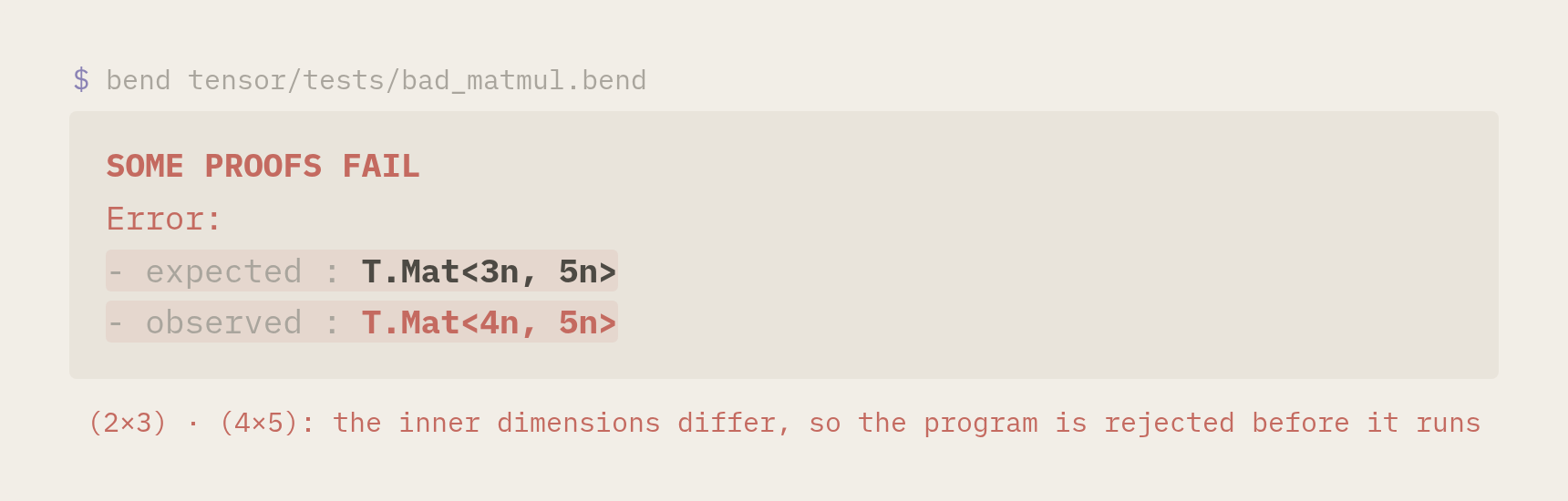
The message says exactly what happened: the second argument should have been Mat<3, 5>, to match the first one's 3 columns, and a Mat<4, 5> arrived.
reshape is more interesting. It rearranges the same numbers into a different shape, say 12 numbers from 2×6 to 3×4. That only makes sense if the total count does not change. In bend-ml, reshape demands a proof of that as an argument:
def Mat.reshape(-r1: Nat, -c1: Nat, r2: Nat, +c2: Nat,
                -p: {Nat.mul(r1, c1) == Nat.mul(r2, c2) : Nat},
                a: Mat<r1, c1>) -> Mat<r2, c2>:
The parameter p has a strange type: {r1*c1 == r2*c2}. A value of that type is a proof that the two products are equal. To call the function, you have to hand over that proof. From 2×6 to 3×4, the proof is just {==}, which means "compute both sides and see that they match": 12 and 12. From 2×6 to 5×3, there is no proof that 12 equals 15, and the compiler refuses. And since the parameter is also erased (-p), the proof costs nothing at run time.
When the dimensions are not fixed numbers, the proof becomes a real law. Transposing r×c into c×r requires knowing that r*c == c*r for any r and c, and that is commutativity of multiplication, which had to be proved first.
The same holds inside training. In backprop, which I explain further down, the gradient of a 784×128 weight matrix W is Xᵀ·dY, and its type is Mat<784, 128>. Asking for that gradient as 128×784, the classic mistake of transposing on the wrong side, does not compile either. The whole MNIST training step is checked this way, layer by layer.
the missing proofs
Since Base has no lemmas, the first published package was not even ML: it was bend-ml-nat-lemmas, with 15 laws about Nat and lists. Commutative and associative addition, commutative, associative and distributive multiplication, identity elements, list concatenation and its length.
Commutativity of addition looks like this:
law add_comm:
  for  a: Nat
  for +b: Nat
  {Nat.add(a, b) == Nat.add(b, a) : Nat}

def add_comm(a, b):
  match a:
    case 0n:
      %add_zero(b) : {_ == Nat.add(b, 0n) : Nat}
      {==}
    case 1n+p:
      %add_succ(b, p) : {1n+Nat.add(p, b) == _ : Nat}
      %add_comm(p, b) : {1n+Nat.add(p, b) == 1n+_ : Nat}
      {==}
It is worth reading line by line, because it is the same structure as every proof in the project.
The law is the statement: for every a and every b, a + b == b + a. I explain the + before b later; for now, it says b may be used more than once.
The def with the same name is the proof. match a splits the two cases of a natural number: either it is zero (0n), or it is "one plus something" (1n+p), where p is the previous number. Those are the two dominoes.
In the zero case, the goal is 0 + b == b + 0. Bend already knows how to simplify the left side to b, but not the right one. %add_zero(b) uses another lemma, b + 0 == b, to rewrite the goal, and then both sides become b and {==} closes it.
In the 1+p case, the goal is (1+p) + b == b + (1+p). %add_succ rewrites the right side to 1 + (b + p). %add_comm(p, b) is the recursive call: the law itself, for the smaller number p. It is the "if it holds for the previous one". It swaps p + b for b + p, both sides become equal, and {==} closes it.
There is no tactic language, as in Lean or Coq: you prove by writing code. Coming from Python like me, reading this for the first time looks like magic; after the tenth proof, it looks like recursion with a very demanding type. The addition and multiplication proofs follow Bend's official numeric-proofs demo, adapted to Base's Nat.add and Nat.mul.
The lemma that mattered most was product_append, which says the product of a concatenated list is the product of each part. A list of dimensions is a tensor's shape, and its product is the number of elements: this lemma is what holds up reshape for arbitrary shapes.
This was also the first package on BendHub. Publishing is one command, but since there is no undo, it became a rule: I only publish after ALL PROOFS CHECK, after --verdict passes, with no @unsafe (the language's "trust me", which turns checking off) and no ?TODO (a hole left for later) in the file, and after importing the package from BendHub itself in a clean folder and using one of its laws.
text becomes numbers: the tokenizer
A language model does not read letters: it reads numbers. So all text going into GPT-2 first goes through a tokenizer, which cuts the text into pieces and swaps each piece for a number. Those pieces are the tokens.
The simplest way would be one token per letter. But then a sentence becomes a huge sequence. The other extreme, one token per word, would need a dictionary with every word of every language. GPT-2 uses a middle ground called BPE (byte pair encoding). It starts with the 256 possible bytes, which can represent any text, and learns merges: the pair of tokens that appears together most often becomes a new token. Then the next most frequent pair, and so on. Common words end up as a single token; rare words stay in pieces.
Type anything and move the slider to watch the training happen:
a + a → aaaa + a → aaaaaa + b → aaab
aaabdaaabac✓ decode(encode(text)) == text
Look at the last line: decoding what was encoded gives the original text back. It seems obvious, but it is exactly the kind of thing that breaks in production, on a strange character, a different rule order, an emoji. And it is the main law of the second package, bend-ml-bpe-tokenizer.
In the package, a token is a raw byte, B{n}, or a token created by the rule with id k, M{k}. The table is a list of rules from oldest to newest, just like GPT-2's merges.txt. And the law is this:
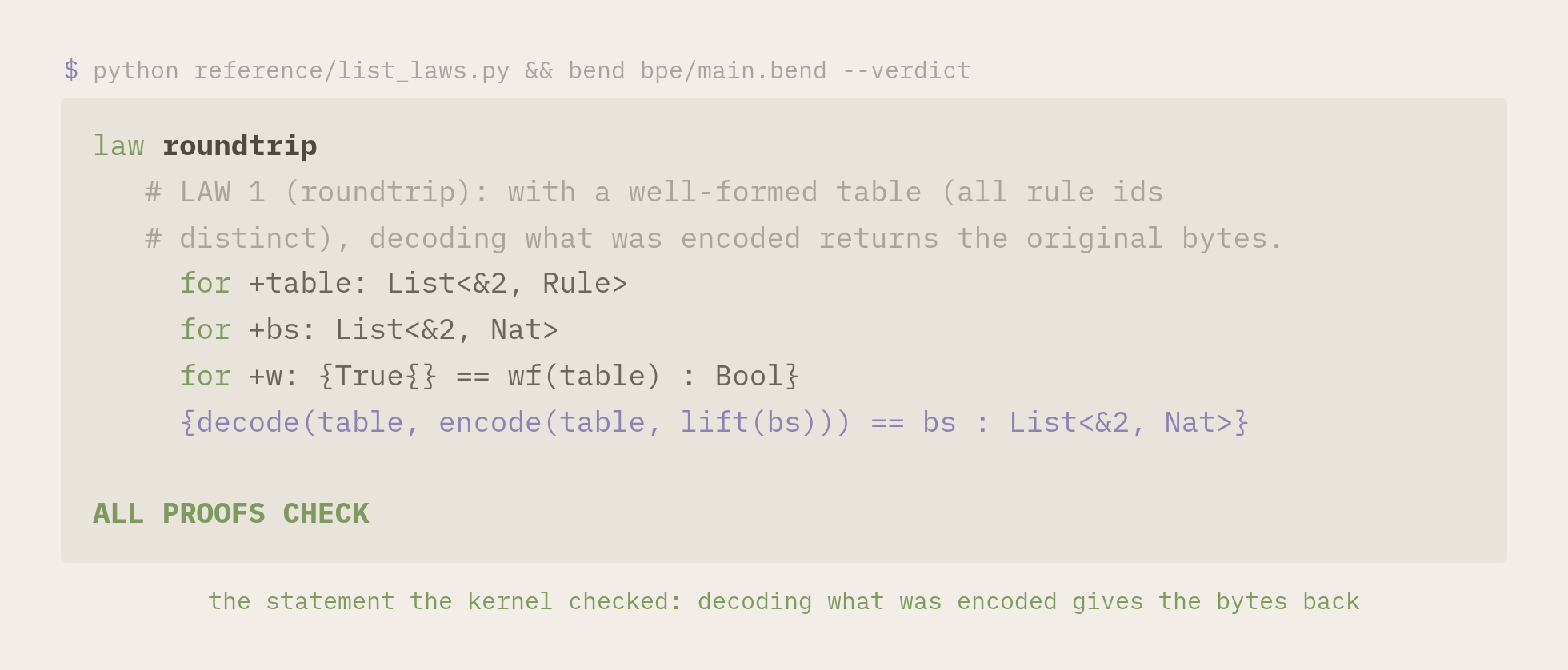
decode(encode(s)) == s, for any byte sequence, as long as the table is well formed, meaning no rule id repeats. The idea of the proof is that when rule k merges the pair (a, b) into M{k}, M{k} expands back to the expansion of a followed by that of b, so decoding changes nothing. That only holds if k did not already exist in the table, which is exactly what "well formed" guarantees. The helper lemmas prove that stacking the new rule on top of the table does not change the expansion of the tokens that already existed.
Alongside it came vocab_bound (every token encode emits is a byte or was created by a rule of the table, never an unknown id) and dec_append (decoding two lists together is decoding each and concatenating the bytes).
Then came the part I like most: proving that train always produces a well-formed table (train_wf). The proof is by induction over the training loop, with the invariant "every id already used is smaller than the next one". An invariant is something that holds before and after every step of a loop; finding the right invariant is half of any proof about loops. Putting the two laws together gives roundtrip_trained: train a table on any corpus, with as many rules as you want, and the roundtrip holds, with no hypothesis at all.
What is not proved is which pair train chooses to merge. And it does not need to be: the roundtrip's correctness does not depend on it. That part is tested against a reference implementation in Python, with English text, accented text (coração, ação), emoji and Chinese characters. train, encode and decode give exactly the same results on both sides.
how a network learns: the gradient
Back to the knobs. To know which way to turn each weight, training computes the gradient: for each weight, how much the error changes if that weight goes up a tiny bit. If raising the weight raises the error, you turn it down; if it lowers the error, you turn it up. It is the slope of the terrain, and training is walking down the hill of error.
Computing the gradient of a function with millions of weights sounds impossible, but there is a trick. Every function in a model is made of small operations (sums, products), chained together. And there is a rule from calculus, the chain rule, that says how to combine the slopes of the parts into the slope of the whole. A framework does this on its own, and that is called automatic differentiation, or autograd.
There are two ways to apply the chain rule. Forward mode carries the slope along with the value, from input to output. Reverse mode computes all the values first and then walks back from the output to the input, handing the gradient backwards. Reverse mode is what every ML framework uses, because in a single pass back it computes the gradient of every weight at once. That is what is called backpropagation.
The third package, bend-ml-autograd, implements both modes and proves they agree. The expression is a tree of constants, the variable, sums and products:
type NE is Data:
  NCst{n: Nat}
  NX{}
  NAdd{a: NE, b: NE}
  NMul{a: NE, b: NE}
Reverse mode receives the gradient g coming from above and hands it to the children. In a product, each side receives g times the value of the other side, exactly as in the diagram:
def nbwd(e: NE, +x: Nat, +g: Nat) -> Nat:
  match e:
    case NCst{n}:
      0n
    case NX{}:
      g
    case NAdd{a, b}:
      Nat.add(nbwd(a, x, g), nbwd(b, x, g))
    case NMul{+a, +b}:
      Nat.add(nbwd(a, x, Nat.mul(g, nval(b, x))), nbwd(b, x, Nat.mul(g, nval(a, x))))
And the law:
law reverse_eq_forward:
  for +e: NE
  for +x: Nat
  {nbwd(e, x, 1n) == nfwd(e, x) : Nat}
The proof goes through a stronger lemma, nbwd(e, x, g) == g * nfwd(e, x) for any g, because the induction only closes if the gradient coming from above is generic. With g = 1, the law follows. It is a common pattern: sometimes the statement you want is not provable directly, but a more general one is.
This is where the rule I wrote at the start of the project, and kept to the end, shows up: floats are not reals. F32 rounds: 0.1 + 0.2 is not exactly 0.3, and addition is not always associative. Proving numeric properties about F32 means trying to prove false things. So the law is proved over Nat, where arithmetic is exact, and the real numbers are tested against PyTorch with gradient checking: you compute the gradient with autograd and compare it with a numeric approximation, nudging the input slightly and measuring the change in the output. Proofs for structure, tests for numbers. That split runs through the whole project.
MNIST: teaching it to read digits
With the packages in place, the two demos came next. The first is machine learning's "hello world": MNIST, a set of 70 thousand photos of handwritten digits, 0 to 9, each 28×28 grayscale pixels. The task is to look at the photo and say which digit it is.
The model is an MLP (multilayer perceptron), the simplest neural network there is. The 784 pixels (28×28) go in, pass through a layer of 128 neurons, and 10 numbers come out, one per digit; the largest is the guess. Each layer is a matrix product plus an adjustment vector (the bias), followed by a function that bends the space, ReLU (which zeroes the negatives).
Training looks at 100 photos at a time, a batch, and the shapes of one step look like this:
X      : Mat<100, 784>     100 photos, 784 pixels each
W1     : Mat<784, 128>     first layer's weights
H = X·W1 + b1 : Mat<100, 128>
W2     : Mat<128, 10>      second layer's weights
Z = H·W2 + b2 : Mat<100, 10>   10 scores per photo

dW2 = Hᵀ·dZ : Mat<128, 10>     the gradient has the weight's shape
dW1 = Xᵀ·dH : Mat<784, 128>
At the end of each step, every weight moves a tiny bit against its gradient (learning rate 0.1). An epoch is going through the 60 thousand training photos once: 600 batches.
To check the result, I made the initial weights in the PyTorch reference script and exported them to Bend, and both sides read the same batches in the same order. That way you can compare number to number, not just "similar accuracy". And it matched: the first epoch's loss is 0.5204771 on both, with 9129 hits out of 10000 test photos. Then 0.27043572 and 9298, then 0.2156194 and 9418. Identical to the seventh digit.
GPT-2: predicting the next word
The second demo is GPT-2 small, the language model OpenAI published in 2019, with 124 million weights. It does one thing: given a text, it predicts the next token. To generate a sentence, you ask for the next token, append it to the text and ask again.
Inside, it is a stack of 12 identical layers, each with two parts. Attention lets each position in the text look at the earlier positions and decide which ones matter (in "the capital of France is", the word "France" matters a lot for what comes next). The MLP transforms the result, as in MNIST. Between the parts come normalizations (LayerNorm) and a smooth function similar to ReLU (GELU).
Getting this to run in Bend took more pieces than I expected:
- the weights come from the official file,
model.safetensors, which a Python script splits into one binary file per tensor. Bend reads each file in blocks withFile.read_atand turns every 4 bytes into anF32. - the tokenizer uses my BPE package with GPT-2's 50 thousand rules. But GPT-2 does not apply the rules in order: it always looks for the pair with the lowest position in the table. I applied them in order and checked against
tiktoken, the official tokenizer, that for trained tables both give the same result. - the pre-tokenizer: before BPE, GPT-2 splits the text with a regular expression that separates contractions, letters, numbers, punctuation and whitespace. Bend has no regular expressions, so I wrote the pre-tokenizer by hand, byte by byte, imitating each alternative of the regex.
- the byte permutation: GPT-2 renumbers the 256 bytes with its own table, which becomes one more file.
- the cache: to avoid recomputing the whole text for each new token, every layer keeps the attention keys and values of the earlier positions, the KV cache.
- generation: greedy, always the highest-scoring token, which is the easiest to compare.
The result: the same tokens as PyTorch, with each token's scores (the logits) equal to the fourth decimal.
$ ./gpt2_fast "The capital of France is" 8
text: The capital of France is the capital of the French Republic, and
(GPT-2 small is not great at geography. But it is wrong in exactly the same way on both sides, which is what matters here.)
v1 worked. and it was 1800 times slower
At the end of the first day, everything was correct and everything was slow.
One MNIST epoch took 544 seconds. PyTorch takes 0.3. About 1800 times slower. GPT-2 took 3 seconds per token, and around 10 seconds just to load the weights.
The temptation was to conclude that Bend is slow and stop there. But I had not measured anything, only timed the total. So v2 started with a different plan: optimize nothing without first having a number that said where the problem was. The second day became a series of experiments, each with a hypothesis and a measurement before any change to the code. All of them are in the project notes, with the command to reproduce them.
why lists are slow
The first suspect was the data structure. v1 stored a matrix as a list of rows, and each row was a linked list: each number sits anywhere in memory, together with the address of the next one. To reach the tenth number, you go through the nine before it.
The alternative is an array: the numbers side by side, and you reach any of them directly by position, the index.
For the processor, the difference is huge. It fetches memory in blocks and tries to guess what you will read next. With an array, the next read sits right next to the previous one and already came in the same block. With a list, each number can be anywhere, and each read waits for the previous one to finish to learn the next address.
Experiment 1. I rewrote the same matrix product (100 million multiply-adds, one thread) with a flat Array<F32>, accessed by index:
| time | multiply-adds/s | |
|---|---|---|
| lists | 2.274 s | 44 M |
Array<F32> by index | 0.046 s | 2,200 M |
Forty-nine times, just by changing the data structure. v1's conclusion ("Bend is 1800 times slower") was an effect of the data structure, not of the language.
Bend's Array has a catch: underneath, it is not a contiguous block of memory, it is a tree, and the index picks the path through the branches. That showed up in two more numbers. Walking the whole tree instead of indexing was 70 times worse. And an array with 2^20 slots instead of 2^17 made the same product 60% slower, because the tree's depth enters every read. The rule that came out of it: allocate the smallest possible array.
affine types, in practice
The array brought in a Bend concept I had only read about: affine values. An affine value can be used at most once. That is what lets Bend manage memory without a garbage collector: if the compiler knows nobody else points to a value, it can free it right away or reuse the space.
For an array, that has a curious consequence: reading an element "uses up" the array. So Array.get returns the element and the array back, so you can keep using it. That leaked into the package's API: every operation returns what it read, together with the result, in a record with its own type. The matrix product returns this:
type MMul<-n: Nat, -k: Nat, -m: Nat> is Type:
  MMul{a: Mat<n, k>, b: Mat<k, m>, c: Mat<n, m>}
Both factors back, and the product. It felt strange for the first hour; after that it felt natural, because it makes explicit who owns each matrix at each point. And the parameter markers complete the story: + allows reusing a Data value (numbers, plain lists), - erases the parameter from the compiled program, and a parameter with no marker can be used only once.
parallelism: when splitting helps and when it hurts
My laptop's processor has 22 threads, meaning it can do 22 things at once. Bend is built for that: it automatically runs in parallel the parts of a program that do not depend on each other. A matrix product is perfect for it, because each row of the result is independent of the others.
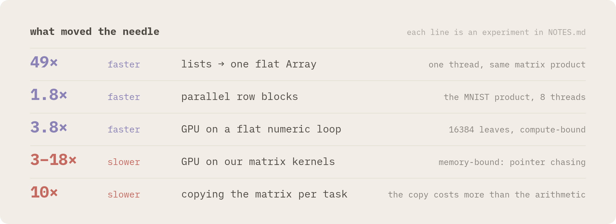
Experiment 2. I split the product into row blocks and sent each block to a task. Since values are affine, each task needs its own copy of the matrices (Array.clone). My hypothesis was that the copies would share memory underneath and the tasks would fight over access. I measured it: 16 tasks reading copies scale exactly like 16 tasks with their own arrays. Hypothesis refuted, and I was glad I measured instead of optimizing for a problem that did not exist. The gain on MNIST was about 2 times.
Experiment 3. In GPT-2, generating one token at a time, the math is matrix times vector: a single input row. I parallelized it the same way and it got 10 times slower, with 1, 8 or 16 threads.
The cause is simple arithmetic. Cloning costs about 0.1 nanoseconds per number, per task. In matrix times vector, each weight is read only once, and the math with it costs about 0.4 nanoseconds. Copying the matrix to several tasks costs more than doing the whole computation alone. In MNIST, matrix times matrix with 100 photos, each weight is read 100 times, and the copy disappears in the noise. I only found that out by measuring.
With the numbers in hand, v2 became a new package, bend-ml-tensor-array: the same Mat<r,c> with the shape in the type, but over a flat Array<F32>, row by row (the number at row i, column j sits at position i*c + j).
A detail I like in it: training needs three different products, X·W (forward), H·Wᵀ and Xᵀ·dZ (backward). Transposing a matrix in memory is expensive. Instead, the package has a single generic product, gemm, which takes the strides the indices walk with in each matrix:
def gemm(+n: Nat, +m: Nat, +k: Nat, +arow: U32, +sa: U32, +sb: U32, +bcol: U32,
         a: Array<F32>, b: Array<F32>, c: Array<F32>) -> G:
The element at row i, position p of A sits at i*arow + p*sa. For a plain A, arow = k and sa = 1. To read A transposed without transposing anything, just swap them: arow = 1 and sa = n. The three public products (matmul, matmul_nt, matmul_tn) are the same gemm with different strides, all three with the right shape in the type. All have optional parallel blocks, and GPT-2 runs its own sequentially, because experiment 3 said so.
In the end, the MNIST epoch went from 544 seconds to about 7 seconds, and GPT-2 from 3 seconds to 0.1 seconds per token.
the GPU looked useless
A graphics card is a different beast. A CPU has a few very smart cores; a GPU has thousands of simple cores that do the same math at the same time on different data. It is perfect for ML, and Bend compiles to CUDA, the platform of NVIDIA cards, when you mark a call with !.
I have an RTX 4050. The first problem was installing: Bend asks for CUDA 12, and my Arch package is 13, which would need sudo and break other things. Digging in, I found that Bend honors the CUDA_HOME variable and only needs two pieces of NVIDIA's kit (cudart and nvrtc). I downloaded the standalone archives, unpacked them into ~/.local/cuda12, and it worked without sudo.
Then came the first result: the GPU was slower than the CPU at everything. From 3 to 18 times, with no point where the curve turned. My first note was "the GPU is useless for this". Rereading it, I found the conclusion too quick: if a GPU loses to the CPU at everything, the likeliest explanation is that I am using it wrong.
I was. Bend's guide says a ! call has to fan out into about 16 thousand leaves, one per GPU execution lane, and end in simple loops, numbers only. My tests used 32 to 1024 tasks: the card sat almost entirely idle. With 16,384 leaves and a simple numeric loop, the GPU won, and the advantage grew with the work per leaf:
16,384 leaves, simple F32 loop | GPU | CPU (22 threads) |
|---|---|---|
| 20 thousand iterations each | 0.217 s | 0.054 s |
| 200 thousand iterations each | 0.254 s | 0.300 s |
| 2 million iterations each | 0.479 s | 1.808 s |
3.8 times faster in the last case. The fixed cost of about 0.2 seconds is compiling the GPU code on the spot.
But the matrix products kept losing, and the reason is beautiful once you see it. Remember the linked list and the array's tree? Each read depends on an address that comes from the previous read. A GPU is great at doing the same math on lots of data that already sits side by side; it is terrible at following addresses. And the memory Bend uses on the GPU is "managed": pages cross the bus between the CPU and the card on first access. Our products are chains of dependent reads, the opposite of what a GPU wants, and that shape of the data is what makes them lose.
The benchmarks stayed on the CPU, with the reason written down. And the first conclusion is still in the notes, corrected instead of erased.
making it stable
Up to that point, everything worked on my machine and on no other. When I asked myself "is this a real v1?", the honest answer was no: a stranger cloning the repository could not run the tests, nothing ran on its own, and the person who wrote the tests was me, the same person who wrote the code. The last part of the work was closing each of those gaps.
To start, make setup && make check on a fresh clone installs Bend pinned to 2.0.35 (checking the binary's SHA256, the file's fingerprint), Lean 4.34.0 for the audited kernel, the Python environment for the references and the MNIST and GPT-2 data, all without sudo. I tested it on a new clone, with an empty HOME, as if I were someone else.
Then CI, GitHub's machine that runs the tests on every change, runs 36 checks on every push, GPT-2 included, on a free runner, in about 11 minutes. Running the full GPT-2 on a free machine was the part I thought would not fit, and it did.
Tests written by the person who wrote the code tend to test what that person already knows works. So randomly generated tests came in: random expression trees for autograd (compared with PyTorch), 80 random corpora for BPE (compared with the Python reference), random shapes for the tensors, and 11 prompts for GPT-2. And a test that imports every package from BendHub, at the version the README states, and applies one of its laws. That one catches a broken publication or a stale README.
For anyone who wants to audit it, a script prints the statement of every law, without the proofs, for anyone who wants to review the specification without reading the implementation. A document lists what is proved, what is tested and what is trusted.
One proof was still missing. The Mat over Array assumed the array had room for r*c numbers. Bend allocates arrays with 2^d slots, and the calculation of d used U32.log2, about which nothing can be proved. I rewrote it with recursion on Nat:
def cap_pair(n: Nat) -> Nat & Nat:
  match n:
    case 0n:
      (0n, 1n)
    case 1n++m:
      cap_step(cap_pair(m), 1n+m)
cap_pair(n) returns the pair (d, 2^d), and each step doubles the power when n no longer fits. With that, the law could be proved:
law cap_ok:
  for +n: Nat
  {True{} == leb(n, pow2(cap_depth(n))) : Bool}
n <= 2^cap_depth(n): the array always has room. What remains trusted is only that the runtime allocates 2^d slots when asked.
Bad inputs now become clear errors. The loss and the hit count gained variants that return None when the number of labels does not match the number of rows, instead of computing garbage. And the tokenizer now validates the rules file before using it: an even number of ids, and no rule referring to a token that does not exist yet:
def ids_ok(ns: List<&2, Nat>, +k: Nat) -> Bool:
  match ns:
    case Nil{}:
      True{}
    case Con{+a, t}:
      match t:
        case Nil{}:
          False{}
        case Con{+b, u}:
          Bool.and(Bool.and(Nat.is_lt(a, Nat.add(256n, k)), Nat.is_lt(b, Nat.add(256n, k))), ids_ok(u, 1n+k))
Rule k may only refer to bytes (below 256) or earlier rules (below 256 + k).
Finally, Unicode. GPT-2's pre-tokenizer treated every byte above 127 as a letter. That worked for accents, but not for em dashes, emoji or Chinese punctuation, which GPT-2's regex treats as "other". The fix: before pre-tokenizing, each byte gets a tag with the class of the character it belongs to, encoded in the number itself:
def tagged(+b: U32, +cls: Nat, +cont: Bool) -> U32:
  U32.add(U32.add(b, U32.mul(U32.from_nat(cls), 256)), U32.mul(U32.from_nat(sel(cont, 1n, 0n)), 2048))
The byte stays in the low 8 bits, the class (letter, number, other, whitespace) in the next bits, and one bit marks the continuation bytes of a multi-byte character. The class comes from a table of 939 Unicode ranges, generated from Python's regex module, with the same categories GPT-2's regex uses. The rest of the pre-tokenizer works on the classes and strips the tags at the end. Result: it matches tiktoken on 79 texts, including 30 strings of random Unicode.
Two stories from this stretch taught me a lot.
The first: the README said that loading GPT-2 used about 10 GB of memory. Measured properly, 10 GB was the address space the process reserved, not memory actually in use; resident memory was 2.3 GB. After reading the weights in 1 MB blocks straight into the array, without building a list in between, it dropped to 1.5 GB, and loading got 5 seconds faster.
The second: after swapping the capacity calculation for the proved version, the MNIST epoch went from 7 to 16 seconds. It looked like the proof had been expensive. I ran the old and new versions side by side: both took 16 seconds. The culprit was my desktop's screensaver, using 134% of a CPU. With the machine idle, it went back to 7. If I had not compared both versions under the same conditions, I would have thrown away a good proof because of a screensaver.
the project's look
The last thing was the README and the video. My first version looked like a generic terminal theme: dark background, saturated blue, cyan and red, macOS-style terminal windows. It was ugly, and I redid it from scratch.
The final version uses Bend's own identity, taken from bend-lang.com's CSS: warm paper (#f2eee7), dark ink, violet as the accent, green for proofs, red for errors. A single monospace font, iA Writer Mono, and the violet cursor blinking after the name, which is their site's signature. The charts follow the site's bar style: vertical, linear scale, Bend in violet and the rest in grey, with the bars that run off the top hatched.
The video at the top of this post is generated too, not recorded. It is an HTML page with a function that draws the frame for a time t; a headless browser takes 3600 screenshots of it and ffmpeg stitches them together, blending frames in pairs for motion blur. Every terminal output and every number in the video is read from the files of the real runs. The 26 cells of the opening matrices travel through the whole film: they become the logo, rearrange in the reshape, become the package boxes, the GPT-2 tokens, the benchmark bars, and return to the logo at the end. make media rebuilds all of it.
where bend got me
A few things I wish I had known on day one:
- affine variables: use something twice, error. The fix is marking the parameter with
+(reuse allowed forDatavalues), or reshaping the code so you do not need to. - structural recursion only: the termination checker requires recursion to visibly shrink something, to guarantee the program ends. When the algorithm does not have that shape, the way out is a "fuel" parameter that shrinks at each step. The pre-tokenizer jumps 1 to 4 bytes at a time (the size of a UTF-8 character), so it takes the number of remaining bytes as fuel, and each step spends one:
def tag(fuel: Nat, +tbl: List<&2, U32>, +xs: List<&2, U32>, +n: Nat, +cls: Nat) -> List<&2, U32>:
  match fuel xs:
    case 1n+p Con{b, t}:
      emit(n, cls, False{}, xs, tag(p, tbl, List.drop(&2, U32, xs, n), ...))
    case _ _:
      Nil{}
matchonly on parameters: you cannotmatchon an expression; it becomes a helper function that receives the already-computed value as an argument.- declaration order: a function can only call another declared before it, and mutual recursion does not pass. More than once the fix was just swapping two functions.
- nested tuple patterns in
matchdo not infer their type. The fix was replacing tuples with records that have their own type, likeMMul. - imports are not re-exported: if a package imports a law from another file, whoever imports the package does not see it. That is why each published package is a single file, with law and proof side by side.
- publishing is forever: a published version cannot be deleted, so every package only went up after all the proofs and the whole test suite passed. The old versions are still there, and the README always points at the current one.
These rules exist for a reason: they are what let Bend manage memory without a garbage collector, guarantee every program terminates and check proofs fast. Still, each one cost me a compile error to understand.
the numbers, no varnish
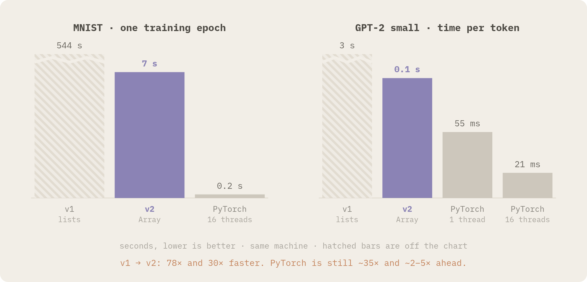
| v1 (lists) | v2 (array) | PyTorch | |
|---|---|---|---|
| MNIST, one epoch | 544 s | ~7 s | 0.2 s |
| GPT-2 small, per token | ~3 s | ~0.1 s | 21 ms (16 threads), 55 ms (1 thread) |
| GPT-2, loading the weights | ~10 s | ~7 s, 1.5 GB | ~1 s |
All measured on the same laptop (Core Ultra 7 155H, 32 GB), with the machine idle; MNIST is the median of three runs. PyTorch is still about 35 times faster on MNIST and 2 to 5 times on GPT-2.
What is left of the gap is in the generated code. Bend 2.0.35 emits scalar code: one operation at a time. Modern processors have SIMD instructions, which do 8 or 16 operations in a single instruction, and PyTorch uses libraries like BLAS, tuned for decades to use every trick the processor has. On the same matrix product, PyTorch does 62 billion multiply-adds per second on one thread; Bend, with an array, 2.3 billion. Closing that gap is compiler work.
what's left
Five packages on BendHub, all MIT, all passing --verdict, with no @unsafe and no ?TODO:
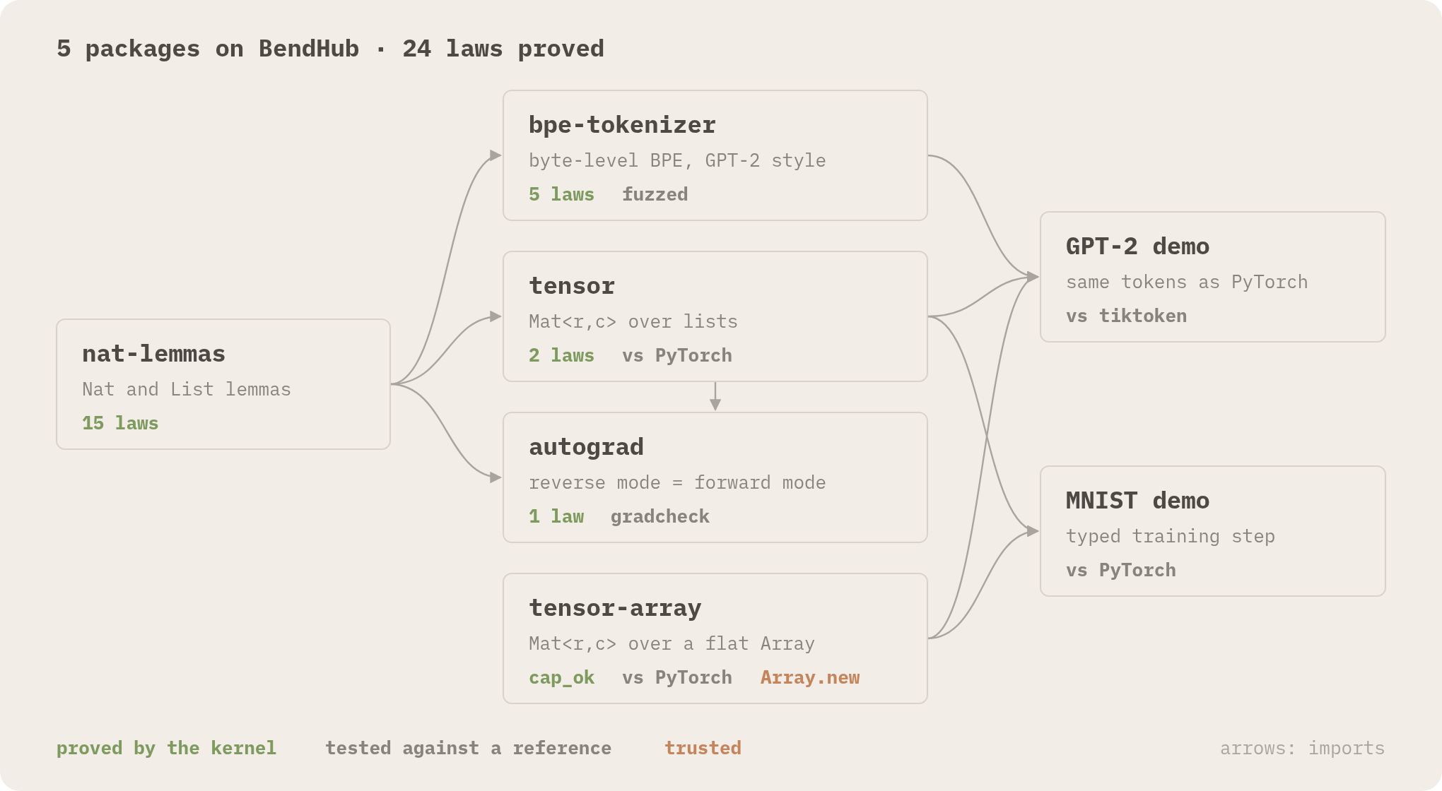
bend-ml-nat-lemmas: 15 laws aboutNatand listsbend-ml-bpe-tokenizer: the tokenizer, withroundtrip,vocab_bound,dec_append,train_wfandroundtrip_trainedbend-ml-tensor:Mat<r,c>over lists, with a provedreshapebend-ml-tensor-array: the same over a flat array, about 50 times faster, withcap_okbend-ml-autograd: automatic differentiation, withreverse_eq_forward
24 laws in total. And what I take from the project, more than the packages:
- types can carry the shapes of a whole training step, including the shape of every gradient, and they cost nothing at run time.
- proofs cover structure, tests cover numbers, and knowing where the line between them runs is half the work.
- the trust base fits in a list: the kernel, the
F32primitives andArray.new. It is written down in the audit guide. - the data structure matters more than the language: the "1800 times slower" was linked lists, not Bend.
- measure before you claim. Three of my conclusions were wrong (PyTorch's time per token, the GPU "slow at everything", the 10 GB of memory), and all three were corrected by a measurement, not by an argument. The corrections stayed in the notes, next to the wrong conclusions.
The obvious next step is splitting the weight array between tasks without copying: since the Array is a tree underneath, its branches can be separated and handed one to each task. That would unlock parallelism in matrix times vector, which today loses to the sequential version. From there to a real llama.bend, the path exists.
The code, the video and all the notes are in the repository. Cloning it, running make setup && make check, and checking every number in this post is the best reply I could get.
Writing this post also made me want to write more about AI here, the same way I did with cryptography: starting from scratch and going deep. Something along those lines is coming soon.
No dia 29 de setembro o Taelin, criador do Bend, publicou um longo despejo sobre o futuro da linguagem. A empresa dele estava levantando uma rodada de investimento, ia montar dois times novos, e no meio do texto tinha uma lista de desejos para o ecossistema. Um item da lista estava escrito assim: "AI framework / PyTorch / llama.bend / etc.".
Alguém perguntou, nas respostas, o que uma pessoa deveria fazer para entrar num desses times. A resposta foi curta: construa alguma coisa em Bend, que mostre tração para os investidores e impressione o time.
Eu já tinha escrito sobre a ideia da linguagem e feito as extensões de editor. Faltava usar de verdade, numa coisa grande. Então peguei o item da lista e passei os dias 3 e 4 de outubro nele. O resultado se chama bend-ml: uma biblioteca de machine learning em Bend, cinco pacotes publicados, um classificador de dígitos escritos à mão e o GPT-2 rodando, tudo com o resultado conferido número a número contra o PyTorch.
Este post é a história inteira. A primeira metade não assume que você sabe nada de machine learning, de tipos ou de provas: eu explico cada peça antes de usar. A segunda metade desce até o código, os experimentos e os números, inclusive os números em que o projeto perde feio.
- 2026-09-19o manifestoescrevo sobre a aposta do bend2 sem ter rodado uma linha.
- 2026-09-29a lista de desejoso taelin publica o despejo: "AI framework / PyTorch / llama.bend".
- 2026-10-03v0.1 a v1.0lemas, tokenizer, tensores, autograd, MNIST e GPT-2. tudo certo, tudo lento.
- 2026-10-04v2 e v2.1os experimentos de performance, a GPU, o CI e as provas que faltavam.
Eu não tenho formação em teoria de tipos nem em provas formais. Meu dia a dia é AI engineering, com agentes e NLP, mas por cima dos modelos: a parte de dentro deles, o treino, os gradientes e os tensores, eu venho estudando por fora. O projeto também foi meu curso intensivo nisso tudo. Quando eu digo "provado" neste post, quem atesta não sou eu: é o checador da linguagem, e qualquer pessoa pode rodar ele de novo.
o que é treinar um modelo
Antes de qualquer código, vale entender o que um framework como o PyTorch faz, porque é isso que eu quis reconstruir.
Um modelo de machine learning é uma função com muitos botões. Você dá uma entrada (a foto de um dígito, um pedaço de texto) e ela devolve uma saída (qual dígito é, qual a próxima palavra). Os botões são números, chamados de pesos, e cada combinação de pesos dá uma função diferente. Treinar é girar esses botões, pouco a pouco, até a função acertar.
O jeito de girar é sempre o mesmo. Você mostra um exemplo, mede o quanto a função errou, descobre para que lado cada botão deveria girar para errar menos, e gira um tiquinho. Depois repete com o próximo exemplo, milhões de vezes. Esse "para que lado girar" é o gradiente, e eu volto nele daqui a pouco.
Os pesos não ficam soltos: ficam organizados em tabelas. Uma tabela de números com linhas e colunas é uma matriz; quando tem mais dimensões, o nome genérico é tensor. E a operação que um modelo faz o tempo inteiro, bilhões de vezes, é multiplicar matrizes.
multiplicar matrizes, e o erro de shape
Multiplicar uma matriz A por uma matriz B é assim: para cada linha de A e cada coluna de B, você multiplica os números um a um e soma tudo. O resultado é um número da matriz C.
Repare na regra escondida aí: para combinar uma linha de A com uma coluna de B número a número, as duas precisam ter o mesmo tamanho. Ou seja, o número de colunas de A tem que ser igual ao número de linhas de B. Uma matriz de 2×3 multiplica uma de 3×4, mas não uma de 4×5. Esse par de números, linhas por colunas, é o shape da matriz.
Num modelo de verdade, os shapes passam por dezenas de camadas, cada uma transformando o shape da anterior. E errar um shape é o bug mais comum de quem escreve modelo. No PyTorch, o erro aparece assim, em tempo de execução, depois que o programa já está rodando:
RuntimeError: mat1 and mat2 shapes cannot be multiplied (2x3 and 4x5)
Às vezes ele aparece em segundos. Às vezes aparece depois de horas de treino, numa camada que só roda no fim de uma época. A pergunta que guiou o projeto foi: e se esse erro nunca pudesse chegar a rodar?
o que é um tipo
Em quase toda linguagem existe a ideia de tipo: a etiqueta que diz que tipo de coisa um valor é. 3 é um inteiro, "olá" é um texto. Em Python os tipos existem, mas ninguém confere antes de rodar: se você soma um número com um texto, o erro só aparece quando aquela linha executa. Em linguagens com checagem estática, um programa chamado checador de tipos lê o código antes de rodar e recusa o que não faz sentido. Somar número com texto nem compila.
Só que o checador de tipos comum não sabe nada de shape. Para ele, uma matriz de 2×3 e uma de 4×5 são do mesmo tipo: "matriz". O erro de shape passa.
O Bend2 tem tipos dependentes. O nome assusta, mas a ideia é simples: um tipo pode depender de um valor. A etiqueta pode carregar números. Então em vez de "matriz", o tipo pode ser "matriz de 2 linhas e 3 colunas", escrito Mat<2, 3>. E aí a regra da multiplicação vira uma regra de tipos: Mat<n, k> vezes Mat<k, m> dá Mat<n, m>, e o k tem que ser o mesmo dos dois lados.
Teste você mesmo. Escolha os shapes de A e B:
Mat<2, 3>Mat<4, 5>—SOME PROOFS FAIL Error: - expected : Mat<3n, 5n> - observed : Mat<4n, 5n>
Um framework em Bend consegue oferecer isso e o PyTorch não, então essa virou a proposta do projeto: um PyTorch onde erro de shape não compila.
o que é uma prova
O Bend2 vai além dos tipos dependentes. Ele tem uma terceira coisa, além de função (def) e dado (type): a lei (law). Uma lei é uma afirmação sobre o programa, do tipo "para todo número a e todo número b, a + b é igual a b + a". E a linguagem exige uma prova de cada lei.
Para quem nunca viu prova formal, a melhor imagem é a de dominós enfileirados. Se você mostra que o primeiro dominó cai, e mostra que qualquer dominó que cai derruba o seguinte, então todos caem, não importa quantos sejam. Isso se chama indução, e é o jeito de provar uma coisa sobre infinitos números com uma quantidade finita de trabalho: você prova para o zero, e prova que se vale para um número, vale para o próximo.
No Bend, uma prova é uma função comum. O tipo da função é a afirmação, e o corpo é o argumento. O caso do zero é o primeiro dominó; a chamada recursiva da função é o "se vale para o anterior". Se a função passa no checador de tipos, a afirmação está provada.
Quem confere isso é o kernel, o pedaço do checador que decide se uma prova está certa. O Bend tem dois: o normal, rápido, e um segundo, chamado com --verdict, que foi escrito e provado correto em Lean, outra linguagem de provas, essa já usada por matemáticos profissionais. O compilador do Bend foi escrito quase todo por IA e não foi auditado inteiro; o kernel do --verdict é a parte que humanos auditaram. Por isso, no projeto, toda lei tinha que passar nos dois.
E aqui entra a tese do Bend: "uma linguagem evoluída por IA, garantida por matemática". Quem escreve o código pode errar; a lei, verificada pelo kernel, garante que certas propriedades valem sempre. ML é exatamente o tipo de código em que ninguém confia muito no que está escrito, e ninguém prova nada.
o reconhecimento
Com a ideia na mão, a primeira tarefa não foi código. O Bend2 é novo e muda rápido, e a sintaxe dele não tem nada a ver com a do Bend1, que era estilo Python. Então eu li a documentação, os exemplos e a biblioteca padrão, e anotei tudo que ia precisar. Algumas descobertas mudaram o plano:
- fixar a versão: tudo foi feito na 2.0.35, e o projeto se recusa a rodar em outra. Numa linguagem que muda toda semana, isso é sobrevivência.
- números: só existem
Nat(naturais: 0, 1, 2...),U32(inteiros de 32 bits) eF32(números com vírgula de 32 bits). Não existeF64. Para ML,F32serve, mas ele volta a aparecer na hora das provas. - a biblioteca padrão quase não tem lemas: o
Basetem números, listas e textos, mas nenhuma prova de que a soma é comutativa, por exemplo. Lema é uma lei pequena, que serve de degrau para provar outras. - o BendHub, o repositório de pacotes: login só pelo GitHub, versões de quatro números (
0.1.2.0), e publicação pública e permanente. Versão publicada não se apaga. - para onde o Bend compila: C, JavaScript e CUDA, que é o que roda em placa de vídeo NVIDIA.
A primeira coisa que eu escrevi foi uma prova de conceito pequena: uma matriz com o shape no tipo, um matmul, e dois programas que não deviam compilar. Quando eles não compilaram, pelo motivo certo, o resto do plano fez sentido.
o shape mora no tipo
Daqui em diante o post fica mais técnico. O tipo central do primeiro pacote, o bend-ml-tensor, é esse:
type Mat<-r: Nat, -c: Nat> is Data:
  Mat{rows: List<&2, List<&2, F32>>}
Uma matriz de r linhas e c colunas guarda uma lista de linhas, cada linha uma lista de F32. O - antes de r e c marca as dimensões como apagadas: elas existem só para o checador e somem do programa compilado. Quer dizer que a garantia não custa nada em tempo de execução. Com isso a multiplicação fica com a assinatura que a matemática pede:
def Mat.matmul(-n: Nat, +k: Nat, +m: Nat, a: Mat<n, k>, b: Mat<k, m>) -> Mat<n, m>:
O k aparece nos dois argumentos. Se a coluna de um não bate com a linha do outro, não existe k que satisfaça, e o programa não compila:
A mensagem diz exatamente o que aconteceu: o segundo argumento devia ser Mat<3, 5>, para casar com as 3 colunas do primeiro, e chegou um Mat<4, 5>.
O reshape é mais interessante. Ele reorganiza os mesmos números num shape diferente, por exemplo 12 números de 2×6 para 3×4. Isso só faz sentido se o total de números não muda. No bend-ml, o reshape exige uma prova disso como argumento:
def Mat.reshape(-r1: Nat, -c1: Nat, r2: Nat, +c2: Nat,
                -p: {Nat.mul(r1, c1) == Nat.mul(r2, c2) : Nat},
                a: Mat<r1, c1>) -> Mat<r2, c2>:
O parâmetro p tem um tipo estranho: {r1*c1 == r2*c2}. Um valor desse tipo é uma prova de que os dois produtos são iguais. Para chamar a função, você precisa entregar essa prova. De 2×6 para 3×4, a prova é só {==}, que significa "computa os dois lados e vê que dá igual": 12 e 12. De 2×6 para 5×3, não existe prova de que 12 é igual a 15, e o compilador recusa. E como o parâmetro também é apagado (-p), a prova não custa nada em tempo de execução.
Quando as dimensões não são números fixos, a prova vira uma lei de verdade. Transpor r×c em c×r exige saber que r*c == c*r para quaisquer r e c, e isso é a comutatividade da multiplicação, que precisou ser provada antes.
O mesmo vale dentro do treino. No backprop, que eu explico mais adiante, o gradiente de uma matriz de pesos W de 784×128 é Xᵀ·dY, e o tipo dele é Mat<784, 128>. Pedir esse gradiente como 128×784, o erro clássico de quem transpõe do lado errado, também não compila. O passo de treino inteiro do MNIST é checado assim, camada por camada.
as provas que faltavam
Como o Base não tem lemas, o primeiro pacote publicado nem foi de ML: foi o bend-ml-nat-lemmas, com 15 leis sobre Nat e listas. Soma comutativa e associativa, multiplicação comutativa, associativa e distributiva, elemento neutro, concatenação de listas e o tamanho dela.
A comutatividade da soma fica assim:
law add_comm:
  for  a: Nat
  for +b: Nat
  {Nat.add(a, b) == Nat.add(b, a) : Nat}

def add_comm(a, b):
  match a:
    case 0n:
      %add_zero(b) : {_ == Nat.add(b, 0n) : Nat}
      {==}
    case 1n+p:
      %add_succ(b, p) : {1n+Nat.add(p, b) == _ : Nat}
      %add_comm(p, b) : {1n+Nat.add(p, b) == 1n+_ : Nat}
      {==}
Vale ler linha por linha, porque é a mesma estrutura de toda prova do projeto.
A law é a afirmação: para todo a e todo b, a + b == b + a. O + antes de b eu explico mais adiante; por enquanto, ele diz que b pode ser usado mais de uma vez.
O def com o mesmo nome é a prova. O match a separa os dois casos de um número natural: ou ele é zero (0n), ou ele é "um mais alguma coisa" (1n+p), onde p é o número anterior. São os dois dominós.
No caso zero, o objetivo é 0 + b == b + 0. O lado esquerdo o Bend já sabe simplificar para b, mas o direito não. O %add_zero(b) usa outro lema, b + 0 == b, para reescrever o objetivo, e aí os dois lados viram b e o {==} fecha.
No caso 1+p, o objetivo é (1+p) + b == b + (1+p). O %add_succ reescreve o lado direito para 1 + (b + p). O %add_comm(p, b) é a chamada recursiva: a própria lei, para o número menor p. É o "se vale para o anterior". Ela troca p + b por b + p, os dois lados ficam iguais, e o {==} fecha.
Não tem linguagem de tática, como no Lean ou no Coq: você prova escrevendo código. Para quem vem de Python como eu, ler isso pela primeira vez parece magia; depois da décima prova, parece só recursão com um tipo muito exigente. As provas de soma e multiplicação seguem a demo oficial de provas numéricas do Bend, adaptadas para o Nat.add e o Nat.mul do Base.
O lema que mais importou foi product_append, que diz que o produto de uma lista concatenada é o produto de cada parte. Uma lista de dimensões é o shape de um tensor, e o produto dela é o número de elementos: é esse lema que sustenta o reshape com shapes arbitrários.
Esse também foi o primeiro pacote no BendHub. Publicar é um comando, mas como não tem volta, virou regra: só publico depois de ALL PROOFS CHECK, de --verdict passar, de não ter nenhum @unsafe (o "confia em mim" da linguagem, que desliga a checagem) nem ?TODO (um buraco deixado para depois) no arquivo, e de importar o pacote do próprio BendHub numa pasta limpa e usar uma lei dele.
texto vira número: o tokenizer
Um modelo de linguagem não lê letras: lê números. Então todo texto que entra no GPT-2 passa antes por um tokenizer, que corta o texto em pedaços e troca cada pedaço por um número. Esses pedaços são os tokens.
O jeito mais simples seria um token por letra. Mas aí uma frase vira uma sequência enorme. O outro extremo, um token por palavra, precisaria de um dicionário com todas as palavras de todas as línguas. O GPT-2 usa um meio-termo chamado BPE (byte pair encoding). Começa com os 256 bytes possíveis, que conseguem representar qualquer texto, e vai aprendendo junções: o par de tokens que mais aparece junto vira um token novo. Depois o próximo par mais frequente, e assim por diante. Palavras comuns acabam virando um token só; palavras raras ficam em pedaços.
Digite qualquer coisa e mexa no controle para ver o treino acontecer:
a + a → aaaa + a → aaaaaa + b → aaab
aaabdaaabac✓ decode(encode(texto)) == texto
Repare na última linha: decodificar o que foi codificado devolve o texto original. Parece óbvio, mas é exatamente o tipo de coisa que quebra em produção, num caractere estranho, numa ordem de regras diferente, num emoji. E é a lei principal do segundo pacote, o bend-ml-bpe-tokenizer.
No pacote, um token é um byte cru, B{n}, ou um token criado pela regra de id k, M{k}. A tabela é uma lista de regras da mais antiga para a mais nova, igual ao merges.txt do GPT-2. E a lei é essa:
decode(encode(s)) == s, para qualquer sequência de bytes, desde que a tabela seja bem formada, ou seja, que nenhum id de regra se repita. A ideia da prova é que, quando a regra k junta o par (a, b) em M{k}, o M{k} expande de volta para a expansão de a seguida da de b, então decodificar não muda nada. Isso só vale se k ainda não existia na tabela, que é justamente o que "bem formada" garante. Os lemas auxiliares provam que colocar a regra nova por cima da tabela não muda a expansão dos tokens que já existiam.
Vieram junto vocab_bound (todo token que o encode emite é um byte ou foi criado por uma regra da tabela, nunca um id desconhecido) e dec_append (decodificar duas listas juntas é decodificar cada uma e concatenar os bytes).
Depois veio a parte que eu mais gosto: provar que o train sempre produz uma tabela bem formada (train_wf). A prova é por indução sobre o laço de treino, com o invariante "todo id já usado é menor que o próximo". Invariante é uma coisa que vale antes e depois de cada passo do laço; achar o invariante certo é metade de qualquer prova sobre laços. Juntando as duas leis, sai roundtrip_trained: treine uma tabela em qualquer corpus, com quantas regras quiser, e o roundtrip vale, sem hipótese nenhuma.
O que não é provado é qual par o train escolhe juntar. E não precisa ser: a correção do roundtrip não depende disso. Essa parte é testada contra uma implementação de referência em Python, com texto em inglês, texto com acento (coração, ação), emoji e caracteres chineses. train, encode e decode dão exatamente o mesmo resultado nos dois lados.
como uma rede aprende: o gradiente
Voltando aos botões. Para saber para que lado girar cada peso, o treino calcula o gradiente: para cada peso, quanto o erro muda se aquele peso aumentar um pouquinho. Se aumentar o peso aumenta o erro, você gira para baixo; se diminui, gira para cima. É a inclinação do terreno, e o treino é descer a ladeira do erro.
Calcular o gradiente de uma função com milhões de pesos parece impossível, mas tem um truque. Toda função de um modelo é feita de operações pequenas (somas, multiplicações), encadeadas. E existe uma regra do cálculo, a regra da cadeia, que diz como combinar as inclinações das partes para ter a inclinação do todo. Um framework faz isso sozinho, e o nome disso é diferenciação automática, ou autograd.
Tem dois jeitos de aplicar a regra da cadeia. O modo direto acompanha a inclinação junto com o valor, da entrada para a saída. O modo reverso calcula todos os valores primeiro e depois volta da saída para a entrada, distribuindo o gradiente para trás. O reverso é o que todo framework de ML usa, porque com uma volta só ele calcula o gradiente de todos os pesos de uma vez. É isso que se chama backpropagation.
O terceiro pacote, o bend-ml-autograd, implementa os dois modos e prova que eles concordam. A expressão é uma árvore de constantes, da variável, de somas e de produtos:
type NE is Data:
  NCst{n: Nat}
  NX{}
  NAdd{a: NE, b: NE}
  NMul{a: NE, b: NE}
O modo reverso recebe o gradiente g que chega de cima e o distribui para os filhos. Numa multiplicação, cada lado recebe g vezes o valor do outro lado, exatamente como no diagrama:
def nbwd(e: NE, +x: Nat, +g: Nat) -> Nat:
  match e:
    case NCst{n}:
      0n
    case NX{}:
      g
    case NAdd{a, b}:
      Nat.add(nbwd(a, x, g), nbwd(b, x, g))
    case NMul{+a, +b}:
      Nat.add(nbwd(a, x, Nat.mul(g, nval(b, x))), nbwd(b, x, Nat.mul(g, nval(a, x))))
E a lei:
law reverse_eq_forward:
  for +e: NE
  for +x: Nat
  {nbwd(e, x, 1n) == nfwd(e, x) : Nat}
A prova passa por um lema mais forte, nbwd(e, x, g) == g * nfwd(e, x) para qualquer g, porque a indução só fecha se o gradiente que chega de cima for genérico. Com g = 1, sai a lei. É um padrão comum: às vezes a afirmação que você quer não é provável direto, mas uma mais geral é.
Aqui aparece a regra que eu escrevi no começo do projeto e mantive até o fim: float não é número real. F32 arredonda: 0.1 + 0.2 não é exatamente 0.3, e a soma nem sempre é associativa. Provar propriedade numérica sobre F32 é pedir para provar coisa falsa. Então a lei é provada sobre Nat, onde a aritmética é exata, e os números de verdade são testados contra o PyTorch, com gradient checking: você calcula o gradiente pelo autograd e confere com uma aproximação numérica, mexendo de leve na entrada e medindo a mudança na saída. Prova para a estrutura, teste para os números. Essa divisão atravessa o projeto inteiro.
MNIST: ensinando a ler dígitos
Com os pacotes no lugar, vieram as duas demos. A primeira é o "hello world" de machine learning: o MNIST, um conjunto de 70 mil fotos de dígitos escritos à mão, de 0 a 9, cada uma com 28×28 pixels em tons de cinza. A tarefa é olhar a foto e dizer qual dígito é.
O modelo é uma MLP (multilayer perceptron), a rede neural mais simples que existe. Os 784 pixels (28×28) entram, passam por uma camada de 128 neurônios, e saem 10 números, um para cada dígito; o maior é o palpite. Cada camada é um produto de matrizes mais um vetor de ajuste (o bias), seguido de uma função que dobra o espaço, a ReLU (que zera os negativos).
O treino olha 100 fotos de cada vez, um batch, e os shapes de um passo ficam assim:
X      : Mat<100, 784>     100 fotos, 784 pixels cada
W1     : Mat<784, 128>     pesos da primeira camada
H = X·W1 + b1 : Mat<100, 128>
W2     : Mat<128, 10>      pesos da segunda camada
Z = H·W2 + b2 : Mat<100, 10>   10 notas por foto

dW2 = Hᵀ·dZ : Mat<128, 10>     o gradiente tem o shape do peso
dW1 = Xᵀ·dH : Mat<784, 128>
No fim de cada passo, cada peso anda um pouquinho contra o gradiente (taxa de aprendizado 0,1). Uma época é passar pelas 60 mil fotos de treino uma vez: 600 batches.
Para conferir o resultado, eu fiz os pesos iniciais no script de referência em PyTorch e exportei para o Bend, e os dois lados leem os mesmos batches na mesma ordem. Assim dá para comparar número com número, não só "acurácia parecida". E bateu: a perda da primeira época é 0.5204771 nos dois, com 9129 acertos em 10000 fotos de teste. Depois 0.27043572 e 9298, depois 0.2156194 e 9418. Igual até a sétima casa.
GPT-2: prevendo a próxima palavra
A segunda demo é o GPT-2 small, o modelo de linguagem que a OpenAI publicou em 2019, com 124 milhões de pesos. Ele faz uma coisa só: dado um texto, prevê o próximo token. Para gerar uma frase, você pede o próximo token, coloca no fim do texto e pede de novo.
Por dentro, ele é uma pilha de 12 camadas iguais, cada uma com duas partes. A atenção deixa cada posição do texto olhar para as posições anteriores e decidir quais importam (em "a capital da França é", a palavra "França" importa muito para o que vem depois). A MLP transforma o resultado, como no MNIST. Entre as partes vêm normalizações (LayerNorm) e uma função suave parecida com a ReLU (GELU).
Fazer isso rodar em Bend exigiu mais peças do que eu imaginava:
- os pesos vêm do arquivo oficial, o
model.safetensors, que um script em Python separa em um arquivo binário por tensor. O Bend lê cada arquivo em blocos comFile.read_ate converte cada 4 bytes em umF32. - o tokenizer usa o meu pacote de BPE com as 50 mil regras do GPT-2. Só que o GPT-2 não aplica as regras em ordem: ele procura sempre o par de menor posição na tabela. Eu apliquei em ordem e conferi contra o
tiktoken, o tokenizer oficial, que para tabelas treinadas as duas coisas dão o mesmo resultado. - o pré-tokenizador: antes do BPE, o GPT-2 quebra o texto com uma expressão regular que separa contrações, letras, números, pontuação e espaços. O Bend não tem expressão regular, então eu escrevi o pré-tokenizador à mão, byte a byte, imitando cada alternativa da regex.
- a permutação dos bytes: o GPT-2 renumera os 256 bytes com uma tabela própria, que vira mais um arquivo.
- o cache: para não recalcular o texto inteiro a cada token novo, cada camada guarda as chaves e valores da atenção das posições anteriores, o KV cache.
- a geração: gulosa, sempre o token de nota mais alta, que é a mais fácil de comparar.
O resultado: os mesmos tokens que o PyTorch, com as notas de cada token (os logits) iguais até a quarta casa.
$ ./gpt2_fast "The capital of France is" 8
text: The capital of France is the capital of the French Republic, and
(O GPT-2 small não sabe geografia muito bem. Mas ele erra igualzinho nos dois lados, que é o que importa aqui.)
a v1 funcionava. e era 1800 vezes mais lenta
No fim do primeiro dia, tudo estava certo e tudo estava lento.
Uma época de MNIST levava 544 segundos. O PyTorch leva 0,3. Umas 1800 vezes mais lento. O GPT-2 levava 3 segundos por token, e uns 10 segundos só para carregar os pesos.
A tentação era concluir que o Bend é lento e parar por ali. Mas eu não tinha medido nada, só cronometrado o total. Então a v2 começou com um plano diferente: não otimizar nada sem antes ter um número que dissesse onde estava o problema. O segundo dia virou uma série de experimentos, cada um com uma hipótese e uma medição antes de qualquer mudança no código. Todos estão nas notas do projeto, com o comando para reproduzir.
por que lista é lenta
O primeiro suspeito era a estrutura de dados. A v1 guardava a matriz como lista de linhas, e cada linha era uma lista encadeada: cada número fica num lugar qualquer da memória, junto com o endereço do próximo. Para chegar no décimo número, você passa pelos nove anteriores.
A alternativa é um array: os números lado a lado, e você chega em qualquer um direto pela posição, o índice.
Para o processador, a diferença é enorme. Ele busca a memória em blocos e tenta adivinhar o que você vai ler depois. Com um array, a próxima leitura está do lado da anterior e já veio no mesmo bloco. Com uma lista, cada número pode estar em qualquer lugar, e cada leitura espera a anterior terminar para saber o endereço da próxima.
Experimento 1. Reescrevi o mesmo produto de matrizes (100 milhões de multiplica-soma, uma thread) com um Array<F32> plano, acessado por índice:
| tempo | multiplica-somas/s | |
|---|---|---|
| listas | 2,274 s | 44 M |
Array<F32> por índice | 0,046 s | 2.200 M |
Quarenta e nove vezes, só trocando a estrutura de dados. A conclusão da v1 ("o Bend é 1800 vezes mais lento") era efeito da estrutura de dados, não da linguagem.
O Array do Bend tem um detalhe: por baixo, ele não é um bloco contínuo de memória, é uma árvore, e o índice escolhe o caminho dos galhos. Isso apareceu em mais dois números. Percorrer a árvore inteira em vez de indexar foi 70 vezes pior. E um array de 2^20 posições em vez de 2^17 deixou o mesmo produto 60% mais lento, porque a profundidade da árvore entra em cada leitura. Regra que saiu disso: alocar o menor array possível.
tipos afins, na prática
O array trouxe um conceito do Bend que eu só tinha lido sobre: valores afins. Um valor afim pode ser usado no máximo uma vez. É isso que deixa o Bend gerenciar memória sem coletor de lixo: se o compilador sabe que ninguém mais aponta para um valor, pode liberar na hora ou reaproveitar o espaço.
Para um array, isso tem uma consequência curiosa: ler um elemento "usa" o array. Então Array.get devolve o elemento e o array de volta, para você continuar usando. Isso vazou para a API do pacote: toda operação devolve o que leu, junto com o resultado, num registro com tipo próprio. O produto de matrizes devolve isso:
type MMul<-n: Nat, -k: Nat, -m: Nat> is Type:
  MMul{a: Mat<n, k>, b: Mat<k, m>, c: Mat<n, m>}
Os dois fatores de volta, e o produto. Estranhei na primeira hora; depois ficou natural, porque deixa explícito quem é dono de cada matriz em cada momento. E os marcadores dos parâmetros completam a história: + permite reusar um valor Data (números, listas comuns), - apaga o parâmetro do programa compilado, e um parâmetro sem marcador pode ser usado uma vez só.
paralelismo: quando dividir ajuda e quando atrapalha
O processador do meu notebook tem 22 threads, ou seja, consegue fazer 22 coisas ao mesmo tempo. O Bend é feito para isso: ele paraleliza automaticamente partes do programa que não dependem umas das outras. Um produto de matrizes é perfeito para isso, porque cada linha do resultado é independente das outras.
Experimento 2. Dividi o produto em blocos de linhas e mandei cada bloco para uma tarefa. Como os valores são afins, cada tarefa precisa da sua própria cópia das matrizes (Array.clone). Minha hipótese era que as cópias compartilhariam memória por baixo e as tarefas iam disputar o acesso. Medi: 16 tarefas lendo cópias escalam igual a 16 tarefas com arrays próprios. Hipótese refutada, e eu fiquei feliz de ter medido em vez de otimizar para um problema que não existia. O ganho no MNIST foi de uns 2 vezes.
Experimento 3. No GPT-2, gerando um token por vez, as contas são matriz vezes vetor: uma linha só de entrada. Paralelizei do mesmo jeito e ficou 10 vezes mais lento, com 1, 8 ou 16 threads.
A causa é aritmética simples. Clonar custa uns 0,1 nanossegundo por número, por tarefa. Em matriz vezes vetor, cada peso é lido uma vez só, e a conta com ele custa uns 0,4 nanossegundo. Copiar a matriz para várias tarefas custa mais que fazer a conta inteira sozinho. No MNIST, matriz vezes matriz com 100 fotos, cada peso é lido 100 vezes, e a cópia some no ruído. Eu só descobri isso medindo.
Com os números na mão, a v2 virou um pacote novo, o bend-ml-tensor-array: o mesmo Mat<r,c> com o shape no tipo, só que sobre um Array<F32> plano, linha por linha (o número da linha i, coluna j fica na posição i*c + j).
Um detalhe que eu gosto nele: o treino precisa de três produtos diferentes, X·W (ida), H·Wᵀ e Xᵀ·dZ (volta). Transpor uma matriz na memória custa caro. Em vez disso, o pacote tem um único produto genérico, o gemm, que recebe os passos com que os índices andam em cada matriz:
def gemm(+n: Nat, +m: Nat, +k: Nat, +arow: U32, +sa: U32, +sb: U32, +bcol: U32,
         a: Array<F32>, b: Array<F32>, c: Array<F32>) -> G:
O elemento da linha i, posição p de A fica em i*arow + p*sa. Para A normal, arow = k e sa = 1. Para ler A transposta sem transpor nada, basta trocar: arow = 1 e sa = n. Os três produtos públicos (matmul, matmul_nt, matmul_tn) são o mesmo gemm com passos diferentes, e os três com o shape certo no tipo. Todos têm blocos paralelos opcionais, e o GPT-2 roda os dele em sequência, porque o experimento 3 mandou.
No fim, a época de MNIST foi de 544 segundos para uns 7 segundos, e o GPT-2 de 3 segundos para 0,1 segundo por token.
a GPU parecia inútil
Placa de vídeo é outro bicho. Uma CPU tem poucos núcleos muito espertos; uma GPU tem milhares de núcleos simples, que fazem a mesma conta ao mesmo tempo em dados diferentes. É perfeita para ML, e o Bend compila para CUDA, a plataforma das placas NVIDIA, marcando uma chamada com !.
Eu tenho uma RTX 4050. O primeiro problema foi instalar: o Bend pede CUDA 12, e o pacote do meu Arch é o 13, que precisaria de sudo e quebraria outras coisas. Investigando, descobri que o Bend respeita a variável CUDA_HOME e só precisa de dois pedaços do kit da NVIDIA (cudart e nvrtc). Baixei os arquivos avulsos, descompactei em ~/.local/cuda12, e funcionou sem sudo.
Aí veio o primeiro resultado: a GPU era mais lenta que a CPU em tudo. De 3 a 18 vezes, sem nenhum ponto em que a curva virasse. Minha primeira anotação foi "a GPU não serve para isso". Relendo, achei a conclusão rápida demais: se uma GPU perde para a CPU em tudo, o mais provável é que eu esteja usando errado.
E estava. O guia do Bend diz que uma chamada ! precisa se abrir em umas 16 mil folhas, uma por linha de execução da GPU, e terminar em laços simples, só com números. Meus testes usavam de 32 a 1024 tarefas: a placa ficava quase toda parada. Com 16.384 folhas e um laço numérico simples, a GPU ganhou, e a vantagem crescia com o trabalho de cada folha:
16.384 folhas, laço simples de F32 | GPU | CPU (22 threads) |
|---|---|---|
| 20 mil iterações cada | 0,217 s | 0,054 s |
| 200 mil iterações cada | 0,254 s | 0,300 s |
| 2 milhões de iterações cada | 0,479 s | 1,808 s |
3,8 vezes mais rápida no último caso. O custo fixo de uns 0,2 segundo é compilar o código da GPU na hora.
Mas os produtos de matriz continuaram perdendo, e o motivo é bonito de entender. Lembra da lista encadeada e da árvore do array? Cada leitura depende de um endereço que vem da leitura anterior. A GPU é ótima para fazer a mesma conta em muitos dados que já estão lado a lado; é péssima para seguir endereços. E a memória que o Bend usa na GPU é "gerenciada": as páginas atravessam o barramento entre a CPU e a placa no primeiro acesso. Nossos produtos são correntes de leituras dependentes, o oposto do que uma GPU quer, e é esse formato dos dados que faz eles perderem.
Os benchmarks ficaram na CPU, com o motivo escrito. E a primeira conclusão continua nas notas, corrigida em vez de apagada.
deixando estável
Até ali, tudo funcionava no meu computador e em nenhum outro. Quando eu me perguntei "isso é uma v1 de verdade?", a resposta honesta foi não: um estranho que clonasse o repositório não conseguiria rodar os testes, nada rodava sozinho, e quem tinha escrito os testes era eu, o mesmo que escreveu o código. A última parte do trabalho foi fechar cada uma dessas lacunas.
Para começar, make setup && make check num clone limpo instala o Bend fixado na 2.0.35 (conferindo o SHA256 do binário, a impressão digital do arquivo), o Lean 4.34.0 para o kernel auditado, o ambiente Python das referências e os dados do MNIST e do GPT-2, tudo sem sudo. Testei num clone novo, com um HOME vazio, como se fosse outra pessoa.
Depois, o CI, a máquina do GitHub que roda os testes a cada mudança, roda 36 checagens a cada push, GPT-2 incluído, num runner gratuito, em uns 11 minutos. Rodar o GPT-2 inteiro numa máquina de graça era a parte que eu achava que não ia caber, e coube.
Testes escritos pela mesma pessoa que escreveu o código tendem a testar o que ela já sabe que funciona. Então entraram testes gerados aleatoriamente: árvores de expressão aleatórias para o autograd (comparadas com o PyTorch), 80 corpora aleatórios para o BPE (comparados com a referência em Python), shapes aleatórios para os tensores, e 11 prompts para o GPT-2. E um teste que importa cada pacote do BendHub, na versão que o README diz, e aplica uma lei dele. Esse pega publicação quebrada ou README desatualizado.
Para quem quiser auditar, um script imprime o enunciado de cada lei, sem as provas, para quem quiser revisar a especificação sem ler a implementação. Um documento lista o que é provado, o que é testado e o que é confiado.
Faltava também uma prova. O Mat sobre Array assumia que o array tinha espaço para r*c números. O Bend aloca arrays com 2^d posições, e o cálculo de d usava U32.log2, sobre o qual não dá para provar nada. Reescrevi o cálculo com recursão em Nat:
def cap_pair(n: Nat) -> Nat & Nat:
  match n:
    case 0n:
      (0n, 1n)
    case 1n++m:
      cap_step(cap_pair(m), 1n+m)
cap_pair(n) devolve o par (d, 2^d), e cada passo dobra a potência quando n não cabe mais. Com isso deu para provar a lei:
law cap_ok:
  for +n: Nat
  {True{} == leb(n, pow2(cap_depth(n))) : Bool}
n <= 2^cap_depth(n): o array sempre tem espaço. O que sobra de confiança é só o runtime alocar 2^d posições quando pedido.
Entradas ruins passaram a virar erro claro. A perda e a contagem de acertos ganharam variantes que devolvem None quando o número de rótulos não bate com o número de linhas, em vez de calcular lixo. E o tokenizer agora valida o arquivo de regras antes de usar: quantidade par de ids, e nenhuma regra citando um token que ainda não existe:
def ids_ok(ns: List<&2, Nat>, +k: Nat) -> Bool:
  match ns:
    case Nil{}:
      True{}
    case Con{+a, t}:
      match t:
        case Nil{}:
          False{}
        case Con{+b, u}:
          Bool.and(Bool.and(Nat.is_lt(a, Nat.add(256n, k)), Nat.is_lt(b, Nat.add(256n, k))), ids_ok(u, 1n+k))
A regra k só pode citar bytes (abaixo de 256) ou regras anteriores (abaixo de 256 + k).
Por fim, o Unicode. O pré-tokenizador do GPT-2 tratava todo byte acima de 127 como letra. Funcionava para acento, mas não para travessão, emoji ou pontuação chinesa, que a regex do GPT-2 trata como "outro". O conserto: antes de pré-tokenizar, cada byte ganha uma etiqueta com a classe do caractere a que ele pertence, codificada no próprio número:
def tagged(+b: U32, +cls: Nat, +cont: Bool) -> U32:
  U32.add(U32.add(b, U32.mul(U32.from_nat(cls), 256)), U32.mul(U32.from_nat(sel(cont, 1n, 0n)), 2048))
O byte fica nos 8 bits de baixo, a classe (letra, número, outro, espaço) nos bits seguintes, e um bit marca os bytes de continuação de um caractere de vários bytes. A classe vem de uma tabela de 939 faixas de Unicode, gerada a partir do módulo regex do Python, com as mesmas categorias que a regex do GPT-2 usa. O resto do pré-tokenizador trabalha com as classes e tira as etiquetas no fim. Resultado: bate com o tiktoken em 79 textos, incluindo 30 strings de Unicode aleatório.
Duas histórias desse trecho me ensinaram bastante.
A primeira: o README dizia que carregar o GPT-2 usava uns 10 GB de memória. Medindo direito, 10 GB era o espaço de endereçamento que o processo reservava, não a memória usada de fato; a memória residente era 2,3 GB. Depois de ler os pesos em blocos de 1 MB direto para o array, sem montar uma lista no meio, caiu para 1,5 GB, e o carregamento ficou 5 segundos mais rápido.
A segunda: depois de trocar o cálculo de capacidade pela versão provada, a época de MNIST foi de 7 para 16 segundos. Parecia que a prova tinha custado caro. Rodei a versão antiga e a nova lado a lado: as duas deram 16 segundos. O culpado era o protetor de tela do meu desktop, usando 134% de CPU. Com a máquina ociosa, voltou para 7. Se eu não tivesse comparado as duas versões nas mesmas condições, teria jogado fora uma prova boa por causa de um screensaver.
a cara do projeto
A última coisa foi o README e o vídeo. A primeira versão que eu fiz tinha cara de tema de terminal genérico: fundo escuro, azul, ciano e vermelho saturados, janelas de terminal estilo macOS. Ficou feio, e eu refiz do zero.
A versão final usa a identidade do próprio Bend, tirada do CSS do bend-lang.com: papel quente (#f2eee7), tinta escura, violeta como acento, verde para prova, vermelho para erro. Uma fonte monoespaçada só, a iA Writer Mono, e o cursor violeta piscando depois do nome, que é a assinatura do site deles. Os gráficos seguem o estilo de barras do site: verticais, escala linear, o Bend em violeta e o resto em cinza, com as barras que passam do topo hachuradas.
O vídeo do começo deste post também é gerado, não gravado. É uma página HTML com uma função que desenha o quadro para um tempo t; um navegador sem interface tira 3600 fotos dela e o ffmpeg junta tudo, mesclando os quadros dois a dois para dar o borrão de movimento. Toda saída de terminal e todo número no vídeo são lidos dos arquivos das execuções reais. As 26 células das matrizes do começo atravessam o filme inteiro: viram o logo, se reorganizam no reshape, viram as caixas dos pacotes, os tokens do GPT-2, as barras do benchmark, e voltam para o logo no fim. make media refaz tudo.
onde o bend me pegou
Algumas coisas que eu gostaria de ter sabido no primeiro dia:
- variáveis afins: usou duas vezes, erro. A saída é marcar o parâmetro com
+(reuso permitido em valoresData), ou reorganizar o código para não precisar. - recursão só estrutural: o checador de terminação exige que a recursão diminua algo visivelmente, para garantir que o programa termina. Quando o algoritmo não tem essa forma, a saída é um parâmetro de "combustível" que diminui a cada passo. O pré-tokenizador pula de 1 a 4 bytes de cada vez (o tamanho de um caractere UTF-8), então ele recebe como combustível o número de bytes que faltam, e cada passo gasta um:
def tag(fuel: Nat, +tbl: List<&2, U32>, +xs: List<&2, U32>, +n: Nat, +cls: Nat) -> List<&2, U32>:
  match fuel xs:
    case 1n+p Con{b, t}:
      emit(n, cls, False{}, xs, tag(p, tbl, List.drop(&2, U32, xs, n), ...))
    case _ _:
      Nil{}
matchsó em parâmetro: não dá para fazermatchnuma expressão; vira uma função auxiliar que recebe o valor já calculado como argumento.- ordem de declaração: uma função só pode chamar outra declarada antes dela, e recursão mútua não passa. Mais de uma vez a correção foi só trocar duas funções de lugar.
- padrões aninhados de tupla em
matchnão inferem tipo. A saída foi trocar tuplas por registros com tipo próprio, como oMMul. - imports não são reexportados: se o pacote importa uma lei de outro arquivo, quem importa o pacote não vê. Por isso cada pacote publicado é um arquivo só, com a lei e a prova lado a lado.
- publicar é para sempre: versão publicada não se apaga, então todo pacote só subia depois de todas as provas e de toda a bateria de testes passarem. As versões antigas continuam lá, e o README sempre aponta para a atual.
Essas regras existem por um motivo: são elas que deixam o Bend gerenciar memória sem coletor de lixo, garantir que todo programa termina e checar provas rápido. Mesmo assim, cada uma me custou um erro de compilação para entender.
os números, sem enfeite
| v1 (listas) | v2 (array) | PyTorch | |
|---|---|---|---|
| MNIST, uma época | 544 s | ~7 s | 0,2 s |
| GPT-2 small, por token | ~3 s | ~0,1 s | 21 ms (16 threads), 55 ms (1 thread) |
| GPT-2, carregar os pesos | ~10 s | ~7 s, 1,5 GB | ~1 s |
Tudo medido no mesmo notebook (Core Ultra 7 155H, 32 GB), com a máquina ociosa; o MNIST é a mediana de três execuções. O PyTorch ainda é umas 35 vezes mais rápido no MNIST e de 2 a 5 vezes no GPT-2.
O que sobra da distância está no código gerado. O Bend 2.0.35 gera código escalar: uma conta por vez. Os processadores modernos têm instruções SIMD, que fazem 8 ou 16 contas numa instrução só, e o PyTorch usa bibliotecas como a BLAS, afinadas há décadas para usar cada truque do processador. No mesmo produto de matrizes, o PyTorch faz 62 bilhões de multiplica-soma por segundo numa thread; o Bend, com array, 2,3 bilhões. Fechar essa distância é trabalho do compilador.
o que ficou
Cinco pacotes no BendHub, todos MIT, todos passando no --verdict, sem nenhum @unsafe e nenhum ?TODO:
bend-ml-nat-lemmas: 15 leis sobreNate listasbend-ml-bpe-tokenizer: o tokenizer, comroundtrip,vocab_bound,dec_append,train_wferoundtrip_trainedbend-ml-tensor:Mat<r,c>sobre listas, comreshapeprovadobend-ml-tensor-array: o mesmo sobre array plano, umas 50 vezes mais rápido, comcap_okbend-ml-autograd: diferenciação automática, comreverse_eq_forward
São 24 leis no total. E o que eu levo do projeto, mais que os pacotes:
- tipos carregam os shapes de um passo de treino inteiro, inclusive o shape de cada gradiente, e não custam nada em tempo de execução.
- prova cobre estrutura, teste cobre número, e saber onde passa a linha entre os dois é metade do trabalho.
- a base de confiança cabe numa lista: o kernel, as primitivas de
F32e oArray.new. Está escrita no guia de auditoria. - a estrutura de dados importa mais que a linguagem: o "1800 vezes mais lento" era lista encadeada, não Bend.
- medir antes de afirmar. Três conclusões minhas estavam erradas (o tempo do PyTorch por token, a GPU "lenta em tudo", os 10 GB de memória), e as três foram corrigidas por uma medição, não por um argumento. As correções ficaram nas notas, do lado das conclusões erradas.
O próximo passo óbvio é dividir o array de pesos entre as tarefas sem copiar: como o Array é uma árvore por baixo, dá para separar os galhos e entregar um para cada tarefa. Isso destravaria o paralelismo em matriz vezes vetor, que hoje perde para a versão sequencial. Daí para um llama.bend de verdade, o caminho existe.
O código, o vídeo e todas as notas estão no repositório. Clonar, rodar make setup && make check, e conferir cada número deste post é a melhor resposta que eu poderia receber.
Inclusive, escrever este post me deu vontade de falar mais sobre IA por aqui, do mesmo jeito que fiz com criptografia: começando do zero e indo fundo. Em breve sai algo nessa linha.